Problem 2.1

Problem 2.1#

Integrated Energy Grids

Problem 2.1

Given the following optimisation problem,

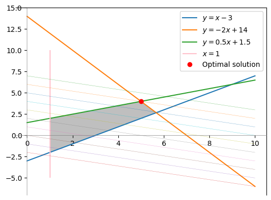
\[\begin{alignat*}{3} \max_{x,y} \quad & 2x + 5y & \\ \text{s.t.} \quad & -x + y & \geq & -3, \\ & 2x + y & \leq & 14, \\ & -\frac{1}{2}x + y & \leq & \frac{3}{2}, \\ & x & \geq & 1. \end{alignat*}\]

a) Solve the optimisation problem graphically (pen and paper or on your laptop). Note that it is a maximisation problem, whereas we will mostly work with minimisations. Reformulate as a minimisation problem.

b) Return to the original formulation. Indicate which constraints are binding and calculate the values of the Lagrange multipliers.

c) In the above set-up, we have a unique solution to our maximisation problem (existence and uniqueness). Adapt the exercise such that this is no longer the case.

a)

We will use numpy to operate with arrays and matplotlib.pyplot to plot the results. We also use linopy to solve linear problems and work with pandas to work with dataframes.

import pandas as pd
import numpy as np
import linopy 
import matplotlib.pyplot as plt

Set parameter Username
Set parameter LicenseID to value 2767832
Academic license - for non-commercial use only - expires 2027-01-20

We define the constraints, and rewrite them in the form y = mx + b. For plotting purposes, we define an evenly spaced sample of the x-values.

x = np.linspace(0, 10, 100)

y0 = x - 3
y1 = -2*x + 14
y2 = 0.5*x + 1.5

# The following will make it easier to fill the area of the feasible space in the graphical solution.

con0 = lambda a: a - 3
con1 = lambda a: -2*a + 14
con2 = lambda a: 0.5*a + 1.5

We will also plot different level sets of the objective function.

fig, ax = plt.subplots()

# Plot the inequalities
ax.plot(x, y0, label=r'$y = x - 3$')
ax.plot(x, y1, label=r'$y = -2x + 14$')
ax.plot(x, y2, label=r'$y = 0.5x + 1.5$')

# Add the constant function
ax.vlines(x=1, ymin=-5, ymax=10, label = r'$x = 1$', color='pink')

# Fill feasible region
z1 = np.linspace(1,5,40)
z2 = np.linspace(5,17/3,40)

ax.fill_between(z1, con0(z1), con2(z1), color='gray', edgecolor=None,alpha=0.5)
ax.fill_between(z2, con0(z2), con1(z2),  color='gray', edgecolor=None,alpha=0.5)

# Plot different level sets of obj.
#opt_val = 30
for val in range(-10, 40, 5):
    y = (val - 2*x)/5
    ax.plot(x, y, ls='--', lw=0.3)

# Plot the optimal solution
ax.plot(5, 4, 'ro', label='Optimal solution')

# Plot the obj
ax.legend();

# Plot the coordinate system
ax.spines['left'].set_position('zero')
ax.spines['left'].set_color('gray')
ax.spines['left'].set_linewidth(0.5)
ax.spines['bottom'].set_position('zero')
ax.spines['bottom'].set_color('gray')
ax.spines['bottom'].set_linewidth(0.5)

../_images/b7fcf86e230f538d22823054efabb29eebc3fd571e3f10f0fde641aea5d9f1f3.png

We can write the problem as a minimisation problem as follows:

\[\begin{alignat*}{3} \min_{x,y} \quad & -2x - 5y & \\ \text{s.t.} \quad & -x + y & \geq & -3, \\ & 2x + y & \leq & 14, \\ & -\frac{1}{2}x + y & \leq & \frac{3}{2}, \\ & x & \geq & 1. \end{alignat*}\]

b)

Set up the problem in linopy:

# For reference:
m21 = linopy.Model()

# Add the variables.
x = m21.add_variables(lower=0,name="x")
y = m21.add_variables(lower=0,name="y")

# Add the constraints and note the sense of the inequality.
m21.add_constraints(-x + y >= -3)
m21.add_constraints(2*x + y <= 14)
m21.add_constraints(-0.5*x + y <= 1.5)
m21.add_constraints(x >= 1)

# Add the objective function and specify it as a maximization problem.
m21.add_objective(2*x + 5*y, sense = "max")

# Solve the maximization problem.
m21.solve(solver_name="gurobi")

m21.solution

Set parameter Username
Set parameter LicenseID to value 2767832
Academic license - for non-commercial use only - expires 2027-01-20
Read LP format model from file /private/var/folders/zg/by4_k0616s98pw41wld9475c0000gp/T/linopy-problem-1br92tli.lp
Reading time = 0.00 seconds
obj: 4 rows, 2 columns, 7 nonzeros
Gurobi Optimizer version 13.0.0 build v13.0.0rc1 (mac64[arm] - Darwin 25.2.0 25C56)

CPU model: Apple M3
Thread count: 8 physical cores, 8 logical processors, using up to 8 threads

Optimize a model with 4 rows, 2 columns and 7 nonzeros (Max)
Model fingerprint: 0x10c518a0
Model has 2 linear objective coefficients
Coefficient statistics:
  Matrix range     [5e-01, 2e+00]
  Objective range  [2e+00, 5e+00]
  Bounds range     [0e+00, 0e+00]
  RHS range        [1e+00, 1e+01]
Presolve removed 1 rows and 0 columns
Presolve time: 0.00s
Presolved: 3 rows, 2 columns, 6 nonzeros

Iteration    Objective       Primal Inf.    Dual Inf.      Time
       0    6.2000000e+01   8.497000e+00   0.000000e+00      0s
       1    3.0000000e+01   0.000000e+00   0.000000e+00      0s

Solved in 1 iterations and 0.01 seconds (0.00 work units)
Optimal objective  3.000000000e+01

<xarray.Dataset> Size: 16B
Dimensions:  ()
Data variables:
    x        float64 8B 5.0
    y        float64 8B 4.0

Print the duals of the optimization problem

c)

Different ways of changing the problem so it no longer has a unique solution:

make it infeasible (e.g. add a constraint \(y \geq 4.1\))
remove uniqueness (e.g. change the objective function to be \(min_{x,y} x\)), get more than one unique solution along the edge in \(x=1\).