Problem 2.3

Problem 2.3#

Integrated Energy Grids

Problem 2.3

We assume the system from Problem 2.2.

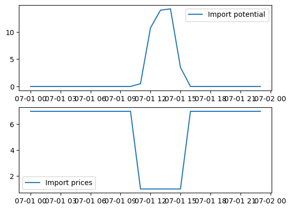
a) Another system that is connected to ours — assuming copper-plate — decides dispatch just before we do and can export utility solar. The results from that dispatch optimization are saved in problem2_3a. Create a time series of available imports and their price.

b) Solve the updated problem with the available imports. Think of the imports as a generator with variable, marginal prices corresponding to the dual variables.

We will use numpy to operate with arrays and matplotlib.pyplot to plot the results. We also use linopy to solve linear problems and work with pandas to work with dataframes.

import pandas as pd
import numpy as np
import linopy 
import matplotlib.pyplot as plt

Set parameter Username
Set parameter LicenseID to value 2767832
Academic license - for non-commercial use only - expires 2027-01-20

a)

Load the data for Problem 3a and also 2c to recreate the system from Problem 2c.

problem2c = pd.read_csv("./data/problem2_2c.csv", index_col=0, parse_dates=True)

problem3a = pd.read_csv("./data/problem2_3a.csv", index_col=0, parse_dates=True)
import_potential = problem3a["utility_solar_potential"] - problem3a["solution.utility_solar"]
import_prices = problem3a["dual.energy_balance"]

Plot import prices and the import potential

fig, ax = plt.subplots(2,1)

ax[0].plot(import_potential, label="Import potential")
ax[1].plot(import_prices, label="Import prices")

ax[0].legend()
ax[1].legend()

<matplotlib.legend.Legend at 0x17ce274d0>

../_images/b1fd25b4c50c1a4339ce9a98ec388cfcdfafa07b9efe630a0a80e19ee7fc1fe6.png

b)

Define the system as before.

# Installed capacities
wind = 15
solar = 20
gas = 20

# Marginal costs (for solar and wind 0)
cost_gas = 60

Set up the model.

m3b = linopy.Model()

time = problem3a.index

x_w = m3b.add_variables(lower=0,name="wind", coords=[time])
x_s = m3b.add_variables(lower=0,name="solar", coords=[time])
x_g = m3b.add_variables(lower=0,name="gas", coords=[time])
x_i = m3b.add_variables(lower=0,name="imports", coords=[time])

# Define constraints
m3b.add_constraints(x_w + x_s + x_g + x_i == problem2c["demand [MWh]"], name="energy_balance")
m3b.add_constraints(x_g <= gas, name="gas_cap")

m3b.add_constraints(x_w <= wind * problem2c["wind cf"], name="wind_cf")
m3b.add_constraints(x_s <= solar * problem2c["solar cf"], name="solar_cf")
m3b.add_constraints(x_i <= import_potential, name="import_cap")

# Optional:
m3b.add_constraints(x_w <= wind, name="wind_cap")
m3b.add_constraints(x_s <= solar, name="solar_cap")

# Objective
m3b.add_objective(cost_gas*x_g + import_prices.values*x_i, sense = "min")

# Solve
m3b.solve(solver_name="gurobi")

Set parameter Username
Set parameter LicenseID to value 2767832
Academic license - for non-commercial use only - expires 2027-01-20
Read LP format model from file /private/var/folders/zg/by4_k0616s98pw41wld9475c0000gp/T/linopy-problem-b4pcx5bt.lp
Reading time = 0.00 seconds
obj: 168 rows, 96 columns, 240 nonzeros
Gurobi Optimizer version 13.0.0 build v13.0.0rc1 (mac64[arm] - Darwin 25.2.0 25C56)

CPU model: Apple M3
Thread count: 8 physical cores, 8 logical processors, using up to 8 threads

Optimize a model with 168 rows, 96 columns and 240 nonzeros (Min)
Model fingerprint: 0xb8c70478
Model has 48 linear objective coefficients
Coefficient statistics:
  Matrix range     [1e+00, 1e+00]
  Objective range  [1e+00, 6e+01]
  Bounds range     [0e+00, 0e+00]
  RHS range        [4e-16, 2e+01]
Presolve removed 167 rows and 93 columns
Presolve time: 0.00s
Presolved: 1 rows, 3 columns, 3 nonzeros

Iteration    Objective       Primal Inf.    Dual Inf.      Time
       0    7.5035000e+03   1.350000e+00   0.000000e+00      0s
       1    7.5062000e+03   0.000000e+00   0.000000e+00      0s

Solved in 1 iterations and 0.00 seconds (0.00 work units)
Optimal objective  7.506200000e+03

('ok', 'optimal')

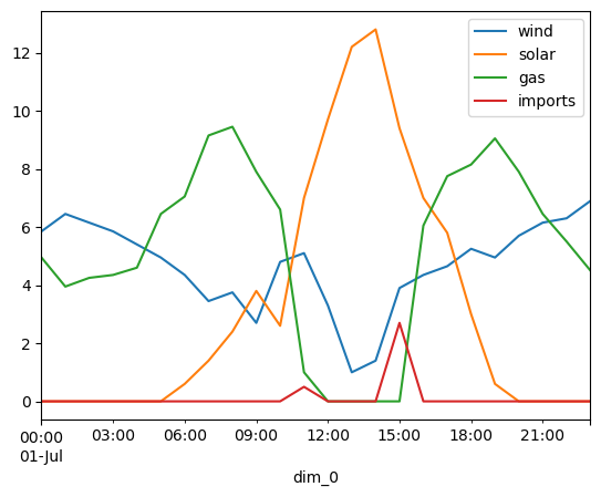
Plot the solution, and print objective value and stats about the electricity price (dual to energy balance)

m3b.solution.to_dataframe().plot()

<Axes: xlabel='dim_0'>

../_images/171e91d47c1119f69b3d78a0b266b3a3856eb2b2af3c157ffe6c62c6597879d8.png

m3b.objective.value/24

312.7583333333333

m3b.dual.energy_balance.to_pandas().describe()

count    24.000000
mean     50.041667
std      22.747153
min       0.000000
25%      60.000000
50%      60.000000
75%      60.000000
max      60.000000
Name: energy_balance, dtype: float64

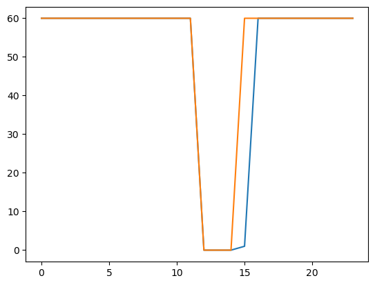
Plot the electricity prices from 2c and 3b. Recreate or copy the results from 2c.

fig, ax = plt.subplots()

ax.plot(m3b.dual.energy_balance, label="Electricity price (3b)")
ax.plot(m22c.dual.energy_balance, label="Electricity price (2c)")

[<matplotlib.lines.Line2D at 0x30440ccd0>]

../_images/44be39a596b5d7c8386be71c4224a49819674bc137d1307653734ed6e14f3016.png